SpaDOT Tutorial

Authors:
Wenjing Ma, Department of Biostatistics, University of Michigan
Siyu Hou, Department of Biostatistics, University of Michigan
Lulu Shang, Department of Biostatistics, MD Anderson Cancer Center
Jiaying Lu, Center for Data Science, School of Nursing, Emory University
Xiang Zhou, Department of Biostatistics, University of Michigan

Maintainer: Wenjing Ma (wenjinma@umich.edu)

Latest revision: 09/30/2025

Table of Contents

• Introduction
• Installation
• Example 1: developing chicken heart
• Conclusion

Introduction

Spatiotemporal transcriptomics is an emerging and powerful approach that adds a temporal dimension to traditional spatial transcriptomics, thus enabling the characterization of dynamic changes in tissue architecture during development or disease progression. Tissue architecture is generally organized into spatial domains – regions within a tissue characterized by relatively similar gene expression profiles that often correspond to distinct biological functions. Crucially, these spatial domains are not static; rather, they undergo complex temporal dynamics during development, differentiation, and disease progression, resulting in emergence, disappearance, splitting, and merging of domains over time. Therefore, we develop SpaDOT (Spatial DOmain Transition detection), a novel and scalable machine learning method for identifying spatial domains and inferring their temporal dynamics in spatiotemporal transcriptomics studies.

(The figure illustrates how SpaDOT works. SpaDOT adopts an integration of two complementary encoders, a Gaussian Process kernel and a Graph Attention Transformer, within one variational autoencoder framework to obtain spatially aware latent representations. The latent representations are further constrained by clustering within each time point and optimal transport (OT) coupling across time points, enabling SpaDOT to identify spatial domains and capture domain transition dynamics. )

In this tutorial, we provide detailed instructions for SpaDOT by utilizing two real data applications: a developing chicken heart sequenced by 10X Vision and a developing mouse brain sequenced by Stereo-seq.

Installation

Step 1: SpaDOT is distributed as a Python package. To get started, please make sure you have Python installed (we recommend Python version >= 3.9). For feature selection, SpaDOT provides a Python implementation of SPARK-X, which we strongly recommend using. Selecting spatially variable genes with SPARK-X has been consistently shown to improve results.

Step 2: Use the following command to install SpaDOT:

pip install SpaDOT

The installation will take seconds to finish and the software dependencies have been taken care of by pip. We have tested our package on Windows, MacOS, and Linux.

You will also have to install your version (based on your pytorch and cuda version) of pyg or torch-sparse and then install torch-geometric, more details can be found here. In my scenario:

pip install pyg-lib torch-scatter torch-sparse -f https://data.pyg.org/whl/torch-2.5.0+cu124.html

pip install torch-geometric -f https://data.pyg.org/whl/torch-2.5.0+cu124.html

Trouble shooting

To make life easier, I would highly recommend using a conda environment.

conda create -n SpaDOT python=3.9
pip install SpaDOT

Then, install pyg-lib and torch-geometric based on your import torch; torch.__version__.

Step 3: If you have successfully installed SpaDOT, you can try the following command:

## Check the help documentation of SpaDOT
SpaDOT -h 

You should see the following console output:

usage: SpaDOT [-h] {preprocess,train,analyze} ...

SpaDOT: Optimal transport modeling uncovers spatial domain dynamics in spatiotemporal transcriptomics.

positional arguments:
  {preprocess,train,analyze}
                        sub-command help.
    preprocess          (Recommended but optional) Perform data preprocessing and feature selection.
    train               Train a SpaDOT model.
    analyze             Analyze the latent representations generated by SpaDOT model.

optional arguments:
  -h, --help            show this help message and exit

In each module, you can use -h to show related help pages. For example, SpaDOT train -h:

usage: SpaDOT train [-h] [-i DATA] [-o OUTPUT_DIR] [--prefix PREFIX] [--config CONFIG] [--device DEVICE] [--save_model]

optional arguments:
  -h, --help            show this help message and exit
  -i DATA, --data DATA  A anndata object containing time point information and spatial coordinates.
  -o OUTPUT_DIR, --output_dir OUTPUT_DIR
                        Output directory to store latent representations. Default: the same as where the data locates.
  --prefix PREFIX       Prefix for output latent representations. Default: ''
  --config CONFIG       Path to the config file, in a yaml format.
  --device DEVICE       Device to use for training. Default: cuda:0
  --save_model          Whether saving the trained model. If specified, the trained model will be stored in the output_dir as 'model.pt'.

Step 4 (Optional): If you prefer using SpaDOT with-in program, you can follow the rendered Jupyter notebooks here.

---

Example 1: developing chicken heart

The developing chicken heart is measured by 10X Visium and collected from four stages: Day 4, Day 7, Day 10 and Day 14. In this dataset, SpaDOT accurately identifies valvulogenesis - a valve splits into artrioventricular valve and semilunar valve at Day 14. For your convenience, you can download the processed data here. If you would like to see the preprocessing steps, please expand the section below:

More details on Chicken Heart data

First, we downloaded the spatial transcritpomics data from GSE149457 and selected

• GSM4502482_chicken_heart_spatial_RNAseq_D4_filtered_feature_bc_matrix.h5
• GSM4502483_chicken_heart_spatial_RNAseq_D7_filtered_feature_bc_matrix.h5
• GSM4502484_chicken_heart_spatial_RNAseq_D10_filtered_feature_bc_matrix.h5
• GSM4502485_chicken_heart_spatial_RNAseq_D14_filtered_feature_bc_matrix.h5

Second, we downloaded spatial coordinates from the analysis code shared by the paper on Github:

• chicken_heart_spatial_RNAseq_D4_tissue_positions_list.csv
• chicken_heart_spatial_RNAseq_D7_tissue_positions_list.csv
• chicken_heart_spatial_RNAseq_D10_tissue_positions_list.csv
• chicken_heart_spatial_RNAseq_D14_tissue_positions_list.csv

Third, we used the script process_ChickenHeart.py provided here to preprocess the data by integrating them into one anndata with timepoint in anndata observations (obs) as one-hot encoder indicating four time points: 0, 1, 2 and 3 indicate Day 4, Day 7, Day 10 and Day 14, respectively. We have also put the spatial coordinates with keyword spatial as a numpy array inside anndata observation metadata (obsm).

After running the process_ChickenHeart.py, we will obtain the file ChickenHeart.h5ad. For your convenience, you can download the processed data here.

Step 1: Perform data preprocessing and feature selection

After obtaining ChickenHeart.h5ad, we perform the data preprocessing. Here, we use command line as demonstration.

SpaDOT preprocess --data ./ChickenHeart.h5ad --output_dir ./ChickenHeart_output

More about no feature selection

If you prefer not to perform spatially variable gene selection, you can add the option --feature_selection False to use all genes in the dataset. However, we still recommend performing feature selection, as it generally leads to better results and faster computation.

SpaDOT preprocess --data ./ChickenHeart.h5ad --feature_selection False --output_dir ./ChickenHeart_output

After data preprocessing, we will have processed_ChickenHeart.h5ad in the directory.

Step 2: Train SpaDOT to obtain latent representations

Then, we can train the SpaDOT model to obtain latent representations by using

SpaDOT train --data ChickenHeart_output/preprocessed_ChickenHeart.h5ad

Here, we train with default parameters. For overriding default parameters purpose, a yaml file is needed. We have provided an example config.yaml with our default parameters for your reference. Again, we do recommend using our default parameters to achieve the best performance, but if you wish to tune them, you can do so with:

SpaDOT train --data ChickenHeart_output/preprocessed_ChickenHeart.h5ad --config config.yaml

The default device is cuda:0. You can switch to CPU by setting the --device option to cpu. However, we recommend training on a GPU, which typically takes around 5 minutes. Training on a CPU is also possible but will take significantly longer.

Step 3: Infer spatial domains and domain dynamics

Once the training stage finishes, we can obtain spatial domains and generate domain dynamics. If we have prior knowledge on how many domains we might have (given by the original study), we can run:

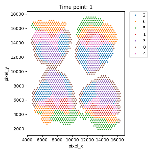
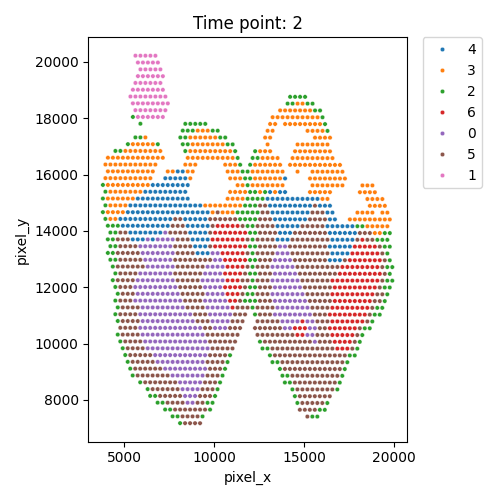
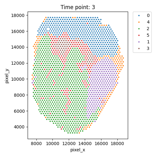
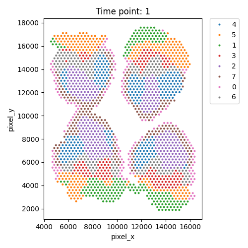
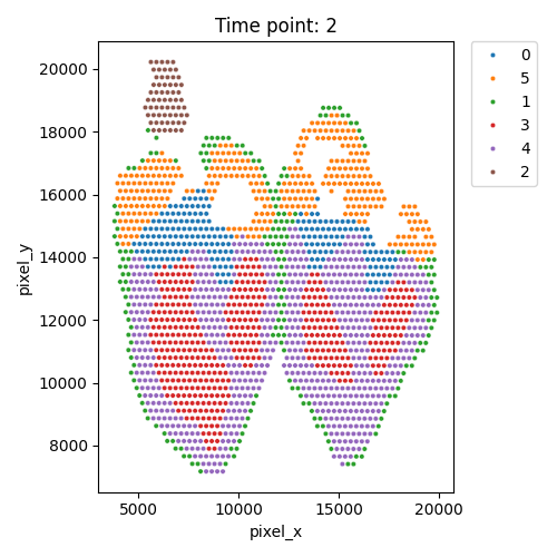
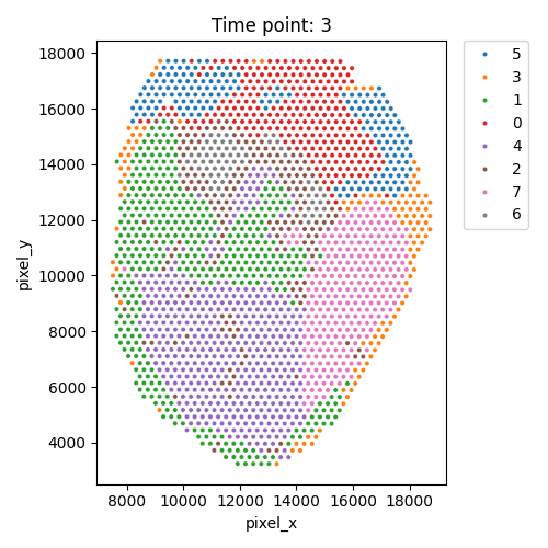
SpaDOT analyze --data ChickenHeart_output/latent.h5ad --n_clusters 5,7,7,6

Output spatial domains

Timepoint	Day 4	Day 7	Day 10	Day 14
Spatial Domains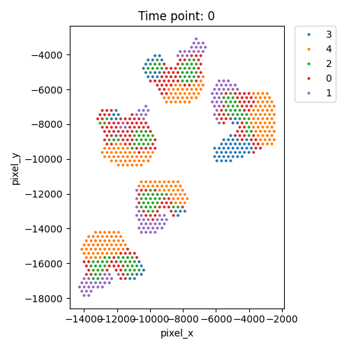

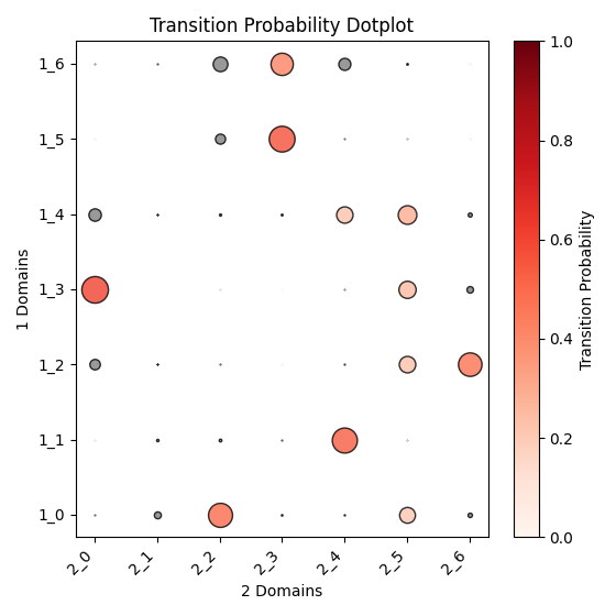
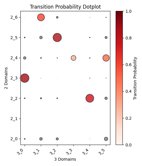
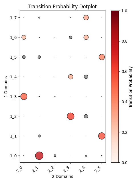
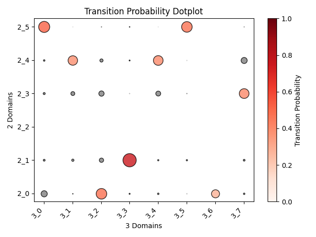
Output OT analysis

Timepoint	Day 4 –> Day 7	Day 7 –> Day 10	Day 10 –> Day 14
OT transition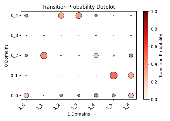

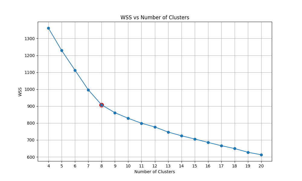
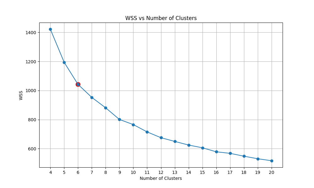
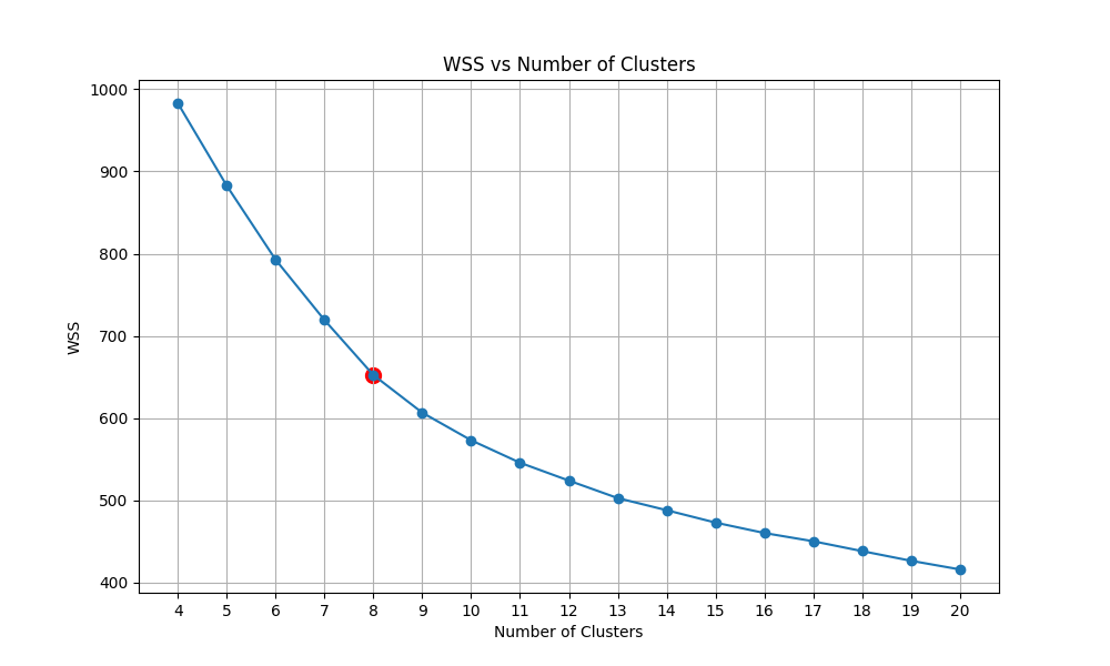
Step 5: infer spatial domains and domain dynamics based on Elbow method (Optional)

Or, we can leave out the --n_clusters option, then SpaDOT would automatically run Elbow method to determine the number of clusters

SpaDOT analyze --data latent.h5ad --prefix adaptive_

We then have the plot of calculating the within-cluster sum of squares (WSS) of KMeans with the number of clusters ranging from 5 to 20. We then detect the Elbow point and select the corresponding cluster number.

Output WSS per cluster and spatial domains

Timepoint	Day 4	Day 7	Day 10	Day 14
WSS per cluster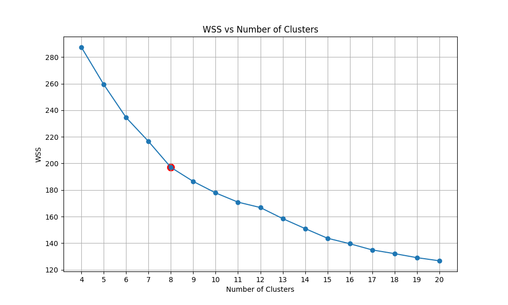
Spatial Domains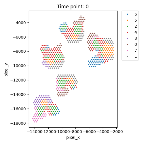

Output OT analysis

Timepoint	Day 4 –> Day 7	Day 7 –> Day 10	Day 10 –> Day 14
OT transition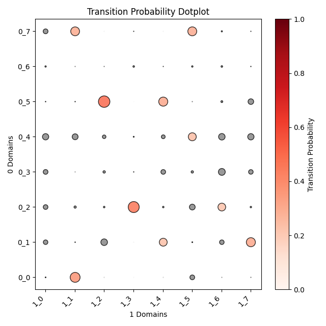

Conclusion

SpaDOT provides efficient and accurate spatial domain detection for spatiotemporal transcriptomics studies and offers insights into domain transition dynamics. Its contributions are three-fold:

1. Capturing domain dynamics via optimal transport (OT) constraints: Across time points, OT constraints guide the alignment of functionally similar domains while separating dissimilar ones, enabling SpaDOT to accurately identify both shared and time-specific domains and infer their biological relationships over time.

2. Modeling both global and local spatial patterns for enhanced structural embedding: Within each time point, SpaDOT integrates a Gaussian Process (GP) prior and Graph Attention Transformer (GAT) within a variational autoencoder (VAE) framework, capturing both global spatial continuity and local structural heterogeneity.

3. Eliminating the need to predefine the number of spatial domains: Unlike existing methods, SpaDOT does not require the number of domains to be specified in advance, reducing dependence on prior knowledge and improving ease of use.

We hope that SpaDOT will be a useful tool for your research. For questions or comments, please open an issue on Github.